House of the Rising Sun ESN example from Herbert Jäger

• Apply RC on vocals of House of the Rising Sun
• Example with output feedback

Problem:

Reservoir states become periodic. Thus, minimization problem yields less effective equations due to linear dependence. Less than the dimension of $\textbf{W}^{out}$ making the system of equations underdetermined. This results in many possible perfect solutions. The ’naive’ solution is unstable. Answer is to add uniform noise to y(n) which results in ’wobbling’ states x(n) around the perfect periodic state sequence used in the naive approach.

Information on notation

import numpy as np
import matplotlib.pyplot as plt
from sklearn.linear_model import Ridge,LinearRegression
from scipy import linalg,stats # for eigenvalue and distribution for sparse connectivity
import sys
sys.path.append("./../")
from utils.timer import *
np.random.seed(42)

Create Data

import musicalbeeps
from midiutil import MIDIFile
import sys
sys.path.append("../")
from utils.periodicList import periodicList

player = musicalbeeps.Player(volume = 0.3,
                            mute_output = True)

# Music theoretically wrong but this is what he uses
# notes = ["g#","a","a#","b","b#","c5","c5#","d5","d5#","e5","e5#","f5","f5#","g5","g5#","a5"]

notes = ["g#","a","bb","b","c5","c5#","d5","e5b","e5","f5","f5#","g5","g5#","a5"]
notes_dict = {i:j for i,j in zip(range(-1,len(notes)-1),notes)}

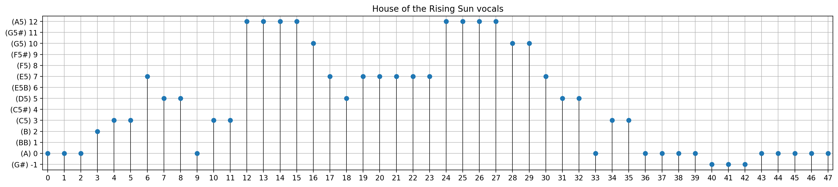
house = 3*[0] + [2] + 2*[3] + [7] + 2*[5] + [0] + 2*[3] + 4*[12] + [10] + [7] + [5] + 5*[7] + 4*[12] \
            + 2*[10] + [7] + 2*[5] + [0] + 2*[3] + 4*[0] + 3*[-1] + 5*[0]

degrees  = [57 + i for i in house]  # MIDI note number
track    = 0
channel  = 0
time_     = 0    # In beats
duration = 0.5    # In beats
tempo    = 220   # In BPM
volume   = 100  # 0-127, as per the MIDI standard

MyMIDI = MIDIFile(1)  # One track, defaults to format 1 (tempo track is created automatically)
MyMIDI.addTempo(track=track,time=time_,tempo=tempo)

for i, pitch in enumerate(degrees):
    MyMIDI.addNote(track, channel, pitch, time_ + i, duration, volume)

with open("house.mid", "wb") as output_file:
    MyMIDI.writeFile(output_file)

# for i in house:
#     player.play_note(notes_dict[i], 0.1)

data = periodicList(house)

Plot

plt.figure(figsize=(20,4),dpi=200)
plt.plot(data[:len(house)],"o")
plt.vlines(range(len(house)),-1.5,data[:len(house)],linewidth=0.7)
plt.title("House of the Rising Sun vocals");
plt.xticks(range(len(house)))
plt.grid(alpha=0.8)
plt.yticks(range(-1,len(notes)-1),[f"({notes_dict[i]}) {i}".upper() for i in range(-1,len(notes)-1)]);
plt.ylim(-1.5,12.5)
plt.xlim(-0.3,47.3);

x0.5 x2

Generate the reservoir

The fact that spectral radius is close to 1 means that the network exhibits a long-lasting response to a unit impulse input. Generally, the closer spectral radius is to unity, the slower is the decay of the network’s response to an impulse input. A relatively long- lasting “echoing” of inputs in the internal network dynamics is a requisite for a sizable short-term memory performance of the network. A substantial short-term memory is required for our present learning task, because the target signal contains a subsequence of 8 consecutive 0’s (namely, the last 5 notes concatenated with the first 3 notes of the subsequent instance of the melody). This implies that the network must realize a memory span of at least 9 update steps in order to correctly produce the first non-0 output after this sequence (from Chapter 4.1.2).

resSize = 400
inSize = outSize = 1

#Creating reservoir-reservoir connections. No input-reservoir connection, since we rely only on outputs (output feedback).
W = 0.1 * stats.rv_discrete(name='sparse', values=([0,4,-4], [0.9875, 0.00625, 0.00625])).rvs(size=(resSize,resSize),random_state=42) 

print('Computing spectral radius...')
rhoW = abs(linalg.eig(W)[0]).max()
print(f'Done: {rhoW}')

Computing spectral radius...
Done: 0.9280529567506998

Output feedback

We do not use any inputs. Since at time n the output y(n) depends on the previous outputs, output feedback is required in this task. The output feedback weights were sampled randomly from the uniform distribution in [−2, 2].

Wback = np.random.uniform(-2,2,size=(resSize,inSize))

"naive" case

Training

trainLen = 1500
initLen = 500 #We initialize the reservoir states
sigmoid = lambda k: 1 / (1 + np.exp(-k))
#Array shapes: (column vector, time)

y_train = np.array(data[:trainLen])/(data.max()*2)
X = np.zeros((resSize,trainLen-initLen)) #to store the echo states
x = np.random.rand(resSize,1)  #reservoir states random init
for t in range(1,trainLen):
    x = sigmoid(np.dot( W, x ) + Wback*y_train[t-1]) #output feedback
    if t >= initLen:
        X[:,t-initLen] = x.ravel()

y_train = np.array(data[initLen:trainLen])/(data.max()*2)

Linear Regression

regr = LinearRegression(fit_intercept=False)
with timer("Linear Regression"):
    regr.fit(X.T,np.arctanh(y_train.T))
    Wout = regr.coef_
print(f"MSE train: {np.square(np.dot(Wout,X)-np.arctanh(y_train)).mean()}")

Linear Regression: 0.042913198471069336 seconds
MSE train: 1.3552039877710011e-20

Plot (naive perfect fit)

plt.figure(figsize=(30,2),dpi=200)
incr = 1
plt.plot(range(0,trainLen-initLen,incr),y_train[::incr],'blue',label='Training Data')
plt.plot(range(0,trainLen-initLen,incr),np.tanh(np.dot(Wout,X)).ravel()[::incr],'r.',alpha = 0.8,label='Fit');
plt.legend(fontsize=15,loc="upper right");
plt.xlim(0,trainLen-initLen);

Test

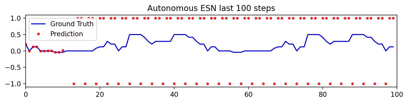
In order to check whether the network has indeed learnt its task, it is tested whether it could stably continue to generate the desired ouputs after a starting period with teacher forcing. The network is started from the null state x(0) = 0, and the correct melody is written into the output units for 500 initial steps. Then the network is left running freely for further 100 steps.

testInitLen = 500
testLen = testInitLen + 100
sigmoid = lambda k: 1 / (1 + np.exp(-k))
#Array shapes: (column vector, time)

y_test = np.array(data[trainLen:trainLen+testLen])/(data.max()*2)
X = np.zeros((resSize,testLen-testInitLen)) #to store the echo states
x = np.zeros((resSize,1))  
for t in range(1,testInitLen):
    x = sigmoid(np.dot( W, x ) + Wback*y_test[t-1]) #output feedback
for t in range(testInitLen,testLen):
    x = sigmoid(np.dot( W, x ) + Wback*np.tanh(np.dot(Wout,x))) #autonomous
    X[:,t-testInitLen] = x.ravel()

Plot (unstable solution)

plt.figure(figsize=(10,2),dpi=200)
incr = 1
plt.plot(range(0,testLen-testInitLen,incr),y_test[testInitLen:][::incr],'blue',label='Ground Truth')
plt.plot(range(0,testLen-testInitLen,incr),np.tanh(np.dot(Wout,X)).ravel()[::incr],'r.',alpha = 0.8,label='Prediction');
plt.legend(fontsize=10,loc="upper left")
plt.xlim(0,testLen-testInitLen)
plt.title("Autonomous ESN last 100 steps");

Reservoir Unit States Plot

plt.figure(figsize=(20,2),dpi=200)
randints = np.random.randint(resSize,size=3)
randints.sort()
plt.plot(X[randints,:].T)
plt.legend(labels=[f"State {i+1}" for i in randints]);

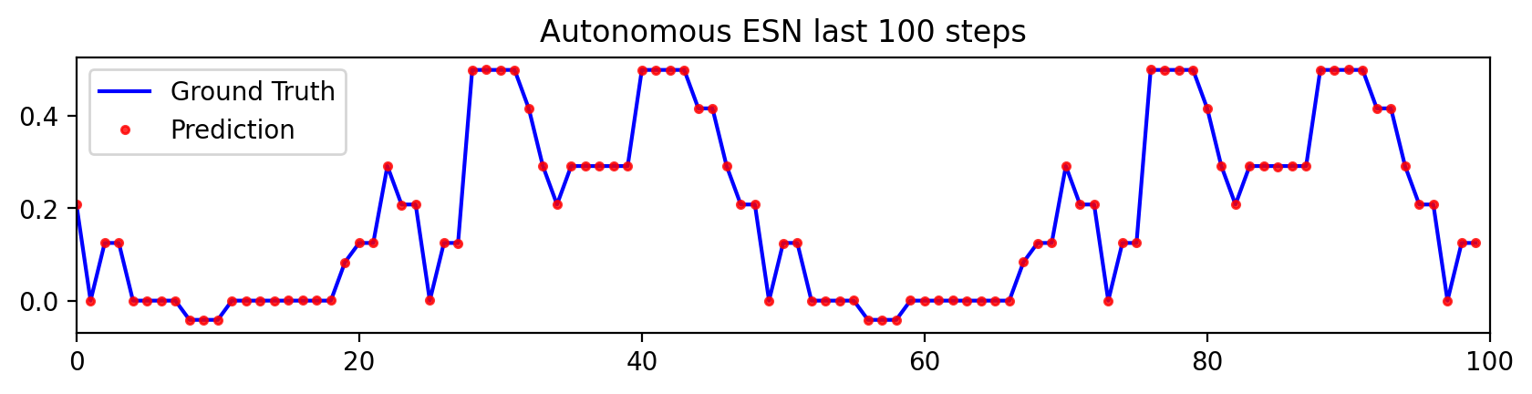
"wobble" case

$x(n + 1) = \sigma(\textbf Wx(n) + \textbf W^{\text {back}}(y(n) + \nu(n))), \nu$: uniform noise

Training

trainLen = 1500
initLen = 500 #We initialize the reservoir states
sigmoid = lambda k: 1 / (1 + np.exp(-k))
#Array shapes: (column vector, time)

y_train = np.array(data[:trainLen])/(data.max()*2)
X = np.zeros((resSize,trainLen-initLen)) #to store the echo states
x = np.random.rand(resSize,1)  #reservoir states random init
for t in range(1,trainLen):
    x = sigmoid(np.dot( W, x ) + Wback*(y_train[t-1]+np.random.uniform(-1,1)/1000)) #output feedback
    if t >= initLen:
        X[:,t-initLen] = x.ravel()

y_train = np.array(data[initLen:trainLen])/(data.max()*2)

Linear Regression

regr = LinearRegression(fit_intercept=False)
with timer("Linear Regression"):
    regr.fit(X.T,np.arctanh(y_train.T))
    Wout = regr.coef_
print(f"MSE train: {np.square(np.dot(Wout,X)-np.arctanh(y_train)).mean()}")

Linear Regression: 0.046041011810302734 seconds
MSE train: 1.4729663638712116e-07

Plot

plt.figure(figsize=(30,2),dpi=200)
incr = 1
plt.plot(range(0,trainLen-initLen,incr),y_train[::incr],'blue',label='Training Data')
plt.plot(range(0,trainLen-initLen,incr),np.tanh(np.dot(Wout,X)).ravel()[::incr],'r.',alpha = 0.8,label='Fit');
plt.legend(fontsize=15,loc="upper right");
plt.xlim(0,trainLen-initLen);

Test

testInitLen = 500
testLen = testInitLen + 100
sigmoid = lambda k: 1 / (1 + np.exp(-k))
#Array shapes: (column vector, time)

y_test = np.array(data[trainLen:trainLen+testLen])/(data.max()*2)
X = np.zeros((resSize,testLen-testInitLen)) #to store the echo states
x = np.zeros((resSize,1))  
for t in range(1,testInitLen):
    x = sigmoid(np.dot( W, x ) + Wback*(y_test[t-1]+np.random.uniform(-1,1)/1000)) #output feedback
for t in range(testInitLen,testLen):
    x = sigmoid(np.dot( W, x ) + Wback*np.tanh(np.dot(Wout,x))) #autonomous
    X[:,t-testInitLen] = x.ravel()

plt.figure(figsize=(10,2),dpi=200)
incr = 1
plt.plot(range(0,testLen-testInitLen,incr),y_test[testInitLen:][::incr],'blue',label='Ground Truth')
plt.plot(range(0,testLen-testInitLen,incr),np.tanh(np.dot(Wout,X)).ravel()[::incr],'r.',alpha = 0.8,label='Prediction');
plt.legend(fontsize=10,loc="upper left");
plt.xlim(0,testLen-testInitLen);
plt.title("Autonomous ESN last 100 steps");

plt.figure(figsize=(20,2),dpi=200)
randints = np.random.randint(resSize,size=3)
randints.sort()
plt.plot(X[randints,:].T)
plt.legend(labels=[f"State {i+1}" for i in randints]);

Comparison with RNN

Now we compare the wobbling ESN to RNN

Importing Tensorflow

import tensorflow as tf
from tensorflow.keras import Model, Sequential
from tensorflow.keras.layers import Dense, Dropout, BatchNormalization, Input, Flatten, LSTM
from tensorflow.keras.optimizers import Adam
from tensorflow.keras.callbacks import EarlyStopping, ModelCheckpoint, ReduceLROnPlateau, Callback, TensorBoard

Create the RNN

model = Sequential()
model.add(LSTM(20, return_sequences=True, input_shape=(1,1)))
model.add(BatchNormalization())
model.add(LSTM(20, return_sequences=False))
model.add(BatchNormalization())
model.add(Dense(10,'relu'))
model.add(BatchNormalization())
model.add(Dense(outSize))
model.compile(optimizer=Adam(lr=0.001), loss='mse')
model.summary()

Model: "sequential"
_________________________________________________________________
Layer (type)                 Output Shape              Param #   
=================================================================
lstm (LSTM)                  (None, 1, 20)             1760      
_________________________________________________________________
batch_normalization (BatchNo (None, 1, 20)             80        
_________________________________________________________________
lstm_1 (LSTM)                (None, 20)                3280      
_________________________________________________________________
batch_normalization_1 (Batch (None, 20)                80        
_________________________________________________________________
dense (Dense)                (None, 10)                210       
_________________________________________________________________
batch_normalization_2 (Batch (None, 10)                40        
_________________________________________________________________
dense_1 (Dense)              (None, 1)                 11        
=================================================================
Total params: 5,461
Trainable params: 5,361
Non-trainable params: 100
_________________________________________________________________

Training

class CustomLogger(Callback):
    def __init__(self, epochs_tot):
        super().__init__()
        self.epochs=epochs_tot
        self.threshold = 1000

    def on_epoch_begin(self, epoch, logs=None):
        self.time_begin = time.time()
    def on_epoch_end(self,epoch,logs=None):
        duration = time.time() - self.time_begin
        if (epoch+1) % self.threshold == 0 or epoch==0:
            print(f"The average {self.model.loss} in epoch {epoch+1} is {logs['loss']:1.8f}. Duration of epoch {epoch+1}: {duration} seconds")
            
epochs = 10000
batch_size = 301
reduceLR = ReduceLROnPlateau(monitor='loss', factor=0.5, patience=epochs//10, min_lr=1e-7, verbose=1)
earlyStopping = EarlyStopping(monitor='loss', patience=epochs//2)
logger = CustomLogger(epochs)
with timer("RNN Training time"):
    history = model.fit(y_train[:,None,None],y_train[:,None,None],batch_size=batch_size,epochs=epochs, verbose=0, callbacks=[earlyStopping,logger])

The average mse in epoch 1 is 0.86838420. Duration of epoch 1: 2.295196056365967 seconds
The average mse in epoch 1000 is 0.00034807. Duration of epoch 1000: 0.01203298568725586 seconds
The average mse in epoch 2000 is 0.00007379. Duration of epoch 2000: 0.013885974884033203 seconds
The average mse in epoch 3000 is 0.00016559. Duration of epoch 3000: 0.02065587043762207 seconds
The average mse in epoch 4000 is 0.00011496. Duration of epoch 4000: 0.010833978652954102 seconds
The average mse in epoch 5000 is 0.00023625. Duration of epoch 5000: 0.01104283332824707 seconds
The average mse in epoch 6000 is 0.00005369. Duration of epoch 6000: 0.010160207748413086 seconds
The average mse in epoch 7000 is 0.00014636. Duration of epoch 7000: 0.010490179061889648 seconds
The average mse in epoch 8000 is 0.00045002. Duration of epoch 8000: 0.011083841323852539 seconds
The average mse in epoch 9000 is 0.00008388. Duration of epoch 9000: 0.014915943145751953 seconds
The average mse in epoch 10000 is 0.00020240. Duration of epoch 10000: 0.011077880859375 seconds
RNN Training time: 120.02705073356628 seconds

Plot

plt.figure(figsize=(30,2),dpi=200)
incr = 1
plt.plot(range(0,len(y_train),incr),y_train[::incr],'blue',label='Ground Truth')
plt.plot(range(0,len(y_train),incr),history.model.predict(y_train[:,None,None])[::incr],'r.',alpha = 0.8,label='Prediction');
plt.legend(fontsize=15,loc="lower left");
plt.xlim(0,len(y_train));

Validation

RNN_val = []; RNN_se_val = []

with timer("RNN Forecast time"):
    pred = history.model.predict(y_test[testInitLen,None,None,None])
    RNN_val.append(*pred.ravel())
    RNN_se_val.append((RNN_val[-1]-y_test[testInitLen])**2)
    
    for i in range(1,testLen-testInitLen):
        pred = history.model.predict(np.expand_dims(pred,2))
        RNN_val.append(*pred.ravel())
        RNN_se_val.append((RNN_val[-1]-y_test[testInitLen:][i])**2)
        
RNN_mse = np.mean(RNN_se_val)
print('MSE validation: ', RNN_mse)

RNN Forecast time: 2.6592061519622803 seconds
MSE validation:  0.5804679855048523

Plot

plt.figure(figsize=(30,4),dpi=200)
incr = 1
plt.plot(range(0,testLen-testInitLen,incr),y_test[testInitLen:][::incr],'blue',label='Ground Truth')
plt.plot(range(0,testLen-testInitLen,incr),RNN_val[::incr],'r.',alpha = 0.8,label='Prediction');
plt.legend(fontsize=15,loc ="lower left");
plt.xlim(0,testLen-testInitLen);