Mackey-Glass ESN from Mantas Lukoševičius and Herbert Jäger

• Apply RC on Mackey-Glass Delay Differential Equations

Information on notation

import numpy as np
import matplotlib.pyplot as plt
from sklearn.linear_model import Ridge,LinearRegression
from scipy import linalg # for eigenvalue
import sys
sys.path.append("./../")
from utils.timer import *
np.random.seed(42)

Import Data

# data = np.loadtxt('./mgdata.txt')[:,1] #1201 data points
data = np.loadtxt('./MackeyGlass_t17.txt') # 10000 data points
print("Data size: ",data.size)
#1-D time series
inSize = outSize = 1
# Training-Validation split
trainval_split=0.8

Data size:  10000

Plot

plt.figure(figsize=(20,5),dpi=200)
plt.plot(data[:1000])
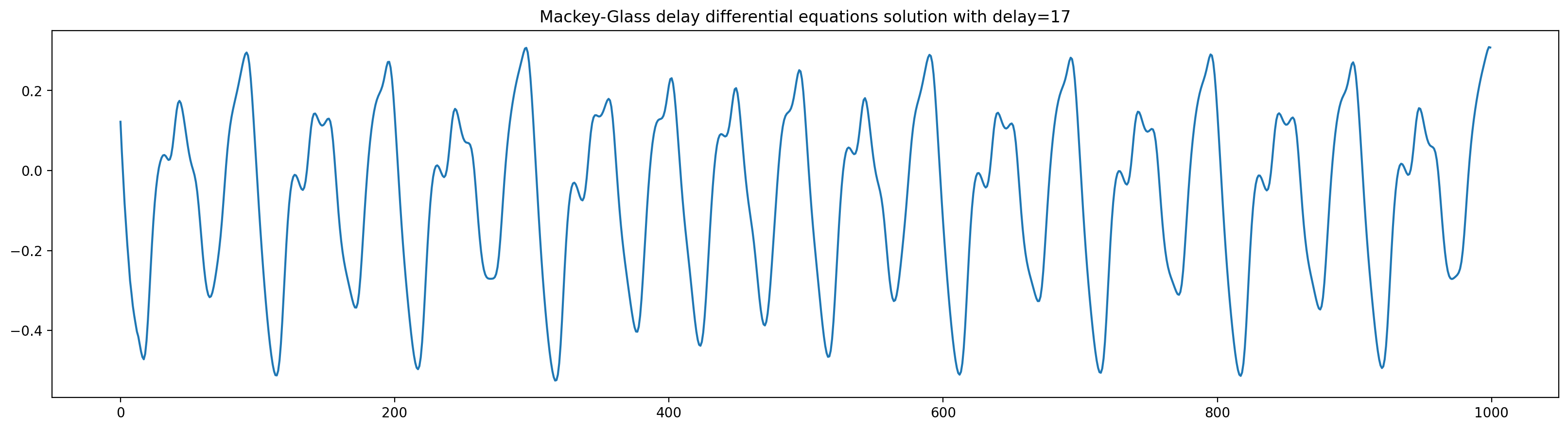
plt.title("Mackey-Glass delay differential equations solution" + bool(data.size>1201)*" with delay=17");

Generate the reservoir

resSize = 1000
alpha = 0.3 # leaking rate

#Creating input-reservoir and reservoir-reservoir connections

Win = np.random.rand(resSize,1+inSize) - 0.5
W = np.random.rand(resSize,resSize) - 0.5 

# normalizing and setting spectral radius (correct, slow):
print('Computing spectral radius...')
rhoW = abs(linalg.eig(W)[0]).max()
print(f'Done: {rhoW}')

desired_spectral_radius = 1.25
print(f'Scaling matrix to have spectral radius {desired_spectral_radius}...')
W *= desired_spectral_radius / rhoW

print('Recalculating spectral radius...')
rhoW = abs(linalg.eig(W)[0]).max()
print(f'Done: {rhoW}')

Computing spectral radius...
Done: 9.204778759016218
Scaling matrix to have spectral radius 1.25...
Recalculating spectral radius...
Done: 1.2499999999999947

Training

We want to predict the next timestep using the previous one. So the training procedure is as follows:

$\textbf{W}^{out} = argmin_\textbf{W} ||y(n) - \textbf{W} \cdot [1;u(n);x(n)]||^2 + \lambda ||\textbf{W}||^2$, where $n \in \mathbb{N}_{train}$ the time indices, $u$ the inputs and $x$ the reservoir states, ";" vertical concatenation, $\lambda$ ridge regularization parameter, $y(n):= u(n+1), u(n) = data(n)$.

Leaking rate $\alpha$

$\alpha$ can be regarded as the time interval in the continuous world between two consecutive time steps in the discrete realization. Small alpha $\rightarrow$ slow dynamics of x(n) $\rightarrow$ longer short term memory.

Recurrent reservoir units $\textbf x(n)$ update rule

$\tilde{\textbf x}(n) = \tanh (\textbf{W}^{in} \cdot [1;u(n)] + \textbf{W} \cdot \textbf x(n − 1)) \\ \textbf x(n) = (1 − α)\textbf x(n − 1) + \alpha \tilde{\textbf x}(n)$

# Here X is the reservoir output, which the readout weights will be trained on via ridge regression
trainLen = int(trainval_split * data.size)
valLen = data.size - trainLen
initLen = 100 #We initialize the reservoir states for 100 timesteps

#Array shapes: (column vector, time)

y_train = data[None,initLen+1:trainLen+1] #+1 since we want the ESN to predict the next timestep using the previous one.
X = np.zeros((1+inSize+resSize,trainLen-initLen)) 
x = np.zeros((resSize,1))  #reservoir states
for t in range(trainLen):
    u = data[t]
    x = (1-alpha)*x + alpha*np.tanh( np.dot( Win, np.vstack((1,u)) ) + np.dot( W, x ) )
    if t >= initLen:
        X[:,t-initLen] = np.vstack((1,u,x)).ravel()

Ridge Regression

regr = Ridge(1e-8, tol=0.1, fit_intercept=False,solver="auto")
with timer("Ridge Regression"):
    regr.fit(X.T,y_train.T)
    Wout = regr.coef_
print(f"MSE train: {((np.dot(Wout,X)-y_train)**2).mean()}")

Ridge Regression: 0.12073183059692383 seconds
MSE train: 2.08200918825242e-09

Plot

plt.figure(figsize=(30,2),dpi=200)
incr = 10
plt.plot(range(0,trainLen-initLen,incr),data[initLen+1:trainLen+1][::incr],'blue',label='Training Data')
plt.plot(range(0,trainLen-initLen,incr),np.dot(Wout,X).ravel()[::incr],'r.',alpha = 0.8,label='Fit');
plt.legend(fontsize=15,loc="upper right");
plt.xlim(0,trainLen-initLen);

Validation

Generative

We use previous states x from the training continuing from where we left off.

Predicted outputs $\hat{y}(n) = \textbf{W}^{out} \cdot [1;u(n);x(n)], n \in \mathbb{N}_{val}$ of the network are used as input for the next time step $u(n+1)$.

X_val = np.zeros((resSize,valLen)) #Just for plotting the reservoir states later on
y_val = np.zeros((outSize,valLen))
errorLen = valLen-1 # We have valLen data points to use for predictions but valLen-1 to compare/validate. 


x = X[2:,-1,None]
u = np.dot( Wout, X[:,-1] )
with timer("RC Forecast time (Generative)"):
    for t in range(valLen-1):
        x = (1-alpha)*x + alpha*np.tanh( np.dot( Win, np.vstack((1,u)) ) + np.dot( W, x ) )
        X_val[:,t] = x.ravel()
        y_val[:,t] = np.dot( Wout, np.vstack((1,u,x)) )
        # generative mode:
        u = y_val[:,t]
        ## this would be predictive mode:
        #u = data[trainLen+t+1] 
    
mse = ((data[trainLen+1:trainLen+errorLen+1] - y_val[:,:errorLen].ravel())**2).mean()
print('MSE validation: ' + str( mse ))

RC Forecast time (Generative): 0.34587717056274414 seconds
MSE validation: 0.033267029188455886

Plot

plt.figure(figsize=(30,4),dpi=200)
incr = 2
plt.plot(range(0,errorLen,incr),data[trainLen+1:trainLen+errorLen+1][::incr],'blue',label='Ground Truth')
plt.plot(range(0,errorLen,incr),y_val[:,:errorLen].ravel()[::incr],'r.',alpha = 0.8,label='Prediction');
plt.legend(fontsize=15,loc="lower left");
plt.xlim(0,errorLen);

Predictive

y_val = np.zeros((outSize,valLen))


x = X[2:,-1,None]
u = data[trainLen]
with timer("RC Forecast time (Predictive)"):
    #We could do valLen predictions but we dont have data to compare the last prediction with.
    for t in range(valLen-1):
        x = (1-alpha)*x + alpha*np.tanh( np.dot( Win, np.vstack((1,u)) ) + np.dot( W, x ) )
        X_val[:,t] = x.ravel()
        y_val[:,t] = np.dot( Wout, np.vstack((1,u,x)) )
        #predictive mode:
        u = data[trainLen+t+1]
        ## this would be generative mode:
        #u = y

mse = ((data[trainLen+1:trainLen+errorLen+1] - y_val[:,:errorLen].ravel())**2).mean()
print('MSE validation: ' + str( mse ))

RC Forecast time (Predictive): 0.35509586334228516 seconds
MSE validation: 2.0358314007445718e-09

Plot

plt.figure(figsize=(30,4),dpi=200)
incr = 2
plt.plot(range(0,errorLen,incr),data[trainLen+1:trainLen+errorLen+1][::incr],'blue',label='Ground Truth')
plt.plot(range(0,errorLen,incr),y_val[:,:errorLen].ravel()[::incr],'r.',alpha = 0.8,label='Prediction');
plt.legend(fontsize=15,loc="lower left");
plt.xlim(0,errorLen);

Reservoir Unit States Plot

plt.figure(figsize=(20,5),dpi=200)
plt.plot(X_val[:10].T)
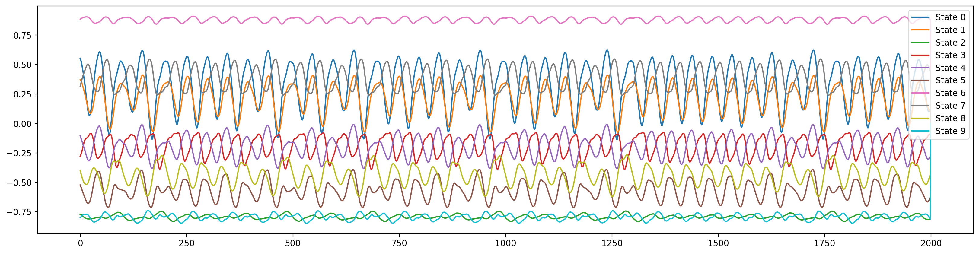
plt.legend(labels=[f"State {i}" for i in range(10)]);

Comparison with RNN

Importing Tensorflow

import tensorflow as tf
from tensorflow.keras import Model, Sequential
from tensorflow.keras.layers import Dense, Dropout, BatchNormalization, Input, Flatten, LSTM
from tensorflow.keras.optimizers import Adam
from tensorflow.keras.callbacks import EarlyStopping, ModelCheckpoint, ReduceLROnPlateau, Callback, TensorBoard

Create the RNN

model = Sequential()
model.add(LSTM(20, return_sequences=True, input_shape=(1,1)))
model.add(BatchNormalization())
model.add(LSTM(20, return_sequences=False))
model.add(BatchNormalization())
model.add(Dense(10,'relu'))
model.add(BatchNormalization())
model.add(Dense(outSize))
model.compile(optimizer=Adam(lr=0.001), loss='mse')
model.summary()

Model: "sequential"
_________________________________________________________________
Layer (type)                 Output Shape              Param #   
=================================================================
lstm (LSTM)                  (None, 1, 20)             1760      
_________________________________________________________________
batch_normalization (BatchNo (None, 1, 20)             80        
_________________________________________________________________
lstm_1 (LSTM)                (None, 20)                3280      
_________________________________________________________________
batch_normalization_1 (Batch (None, 20)                80        
_________________________________________________________________
dense (Dense)                (None, 10)                210       
_________________________________________________________________
batch_normalization_2 (Batch (None, 10)                40        
_________________________________________________________________
dense_1 (Dense)              (None, 1)                 11        
=================================================================
Total params: 5,461
Trainable params: 5,361
Non-trainable params: 100
_________________________________________________________________

Training

Optimization Problem: $argmin_{\theta} ||\text{RNN}^\theta(data(n)) - data(n+1)||,n \in \mathbb{N}_{train}$

class CustomLogger(Callback):
    def __init__(self, epochs_tot):
        super().__init__()
        self.epochs=epochs_tot
        self.threshold = 20

    def on_epoch_begin(self, epoch, logs=None):
        self.time_begin = time.time()
    def on_epoch_end(self,epoch,logs=None):
        duration = time.time() - self.time_begin
        if (epoch+1) % self.threshold == 0 or epoch==0:
            print(f"The average {self.model.loss} in epoch {epoch+1} is {logs['loss']:1.8f}. Duration: {duration} seconds")
            
epochs = 500
batch_size = 1024
reduceLR = ReduceLROnPlateau(monitor='loss', factor=0.5, patience=epochs//10, min_lr=1e-7, verbose=1)
earlyStopping = EarlyStopping(monitor='loss', patience=epochs//2)
logger = CustomLogger(epochs)
with timer("RNN Training time"):
    history = model.fit(data[:trainLen,None,None],data[1:trainLen+1,None,None],batch_size=batch_size,epochs=epochs, verbose=0, callbacks=[earlyStopping,logger])

mse in epoch 1 is 0.21099700. Duration: 2.130035877227783 seconds
mse in epoch 20 is 0.00251189. Duration: 0.03794598579406738 seconds
mse in epoch 40 is 0.00216522. Duration: 0.0415651798248291 seconds
mse in epoch 60 is 0.00190022. Duration: 0.038086891174316406 seconds
mse in epoch 80 is 0.00153878. Duration: 0.03940892219543457 seconds
mse in epoch 100 is 0.00122162. Duration: 0.038205862045288086 seconds
mse in epoch 120 is 0.00127594. Duration: 0.03798198699951172 seconds
mse in epoch 140 is 0.00120943. Duration: 0.040390729904174805 seconds
mse in epoch 160 is 0.00123253. Duration: 0.037442922592163086 seconds
mse in epoch 180 is 0.00121633. Duration: 0.03769803047180176 seconds
mse in epoch 200 is 0.00114664. Duration: 0.040014028549194336 seconds
mse in epoch 220 is 0.00120565. Duration: 0.038513898849487305 seconds
mse in epoch 240 is 0.00117108. Duration: 0.037663936614990234 seconds
mse in epoch 260 is 0.00118534. Duration: 0.03788495063781738 seconds
mse in epoch 280 is 0.00112458. Duration: 0.03818321228027344 seconds
mse in epoch 300 is 0.00110309. Duration: 0.039183855056762695 seconds
mse in epoch 320 is 0.00113553. Duration: 0.03831076622009277 seconds
mse in epoch 340 is 0.00108832. Duration: 0.03792691230773926 seconds
mse in epoch 360 is 0.00116472. Duration: 0.03977704048156738 seconds
mse in epoch 380 is 0.00109350. Duration: 0.03862118721008301 seconds
mse in epoch 400 is 0.00106720. Duration: 0.03889775276184082 seconds
mse in epoch 420 is 0.00112755. Duration: 0.03956794738769531 seconds
mse in epoch 440 is 0.00107194. Duration: 0.038419246673583984 seconds
mse in epoch 460 is 0.00111661. Duration: 0.03842878341674805 seconds
mse in epoch 480 is 0.00109301. Duration: 0.038761138916015625 seconds
mse in epoch 500 is 0.00103337. Duration: 0.03846096992492676 seconds
RNN Training time: 21.97814702987671 seconds

Plot

plt.figure(figsize=(30,2),dpi=200)
incr = 10
plt.plot(range(0,trainLen,incr),data[1:trainLen+1][::incr],'blue',label='Ground Truth')
plt.plot(range(0,trainLen,incr),history.model.predict(data[:trainLen,None,None])[::incr],'r.',alpha = 0.8,label='Prediction');
plt.legend(fontsize=15,loc="lower left");
plt.xlim(0,trainLen);

Validation

Generative

We take a generative approach same as in the case of RC, i.e. the model will predict based on previous predictions of itself.

RNN_val = []; RNN_se_val = []

with timer("RNN Forecast time (Generative)"):
    pred = history.model.predict(data[trainLen,None,None,None])
    RNN_val.append(*pred.ravel())
    RNN_se_val.append((RNN_val[-1]-data[trainLen+1:][0])**2)
    
    for i in range(1,errorLen):
        pred = history.model.predict(np.expand_dims(pred,2))
        RNN_val.append(*pred.ravel())
        RNN_se_val.append((RNN_val[-1]-data[trainLen+1:][i])**2)
        
RNN_mse = np.mean(RNN_se_val)
print('MSE validation: ', RNN_mse)

RNN Forecast time (Generative): 35.36306285858154 seconds
MSE validation:  0.08022835596233922

Plot

plt.figure(figsize=(30,4),dpi=200)
incr = 2
plt.plot(range(0,errorLen,incr),data[trainLen+1:trainLen+errorLen+1][::incr],'blue',label='Ground Truth')
plt.plot(range(0,errorLen,incr),RNN_val[::incr],'r.',alpha = 0.8,label='Prediction');
plt.legend(fontsize=15,loc ="lower left");
plt.xlim(0,errorLen);

Predictive

Now we take a predictive approach, i.e. the model will predict based on data at previous timestep to forecast the next.

with timer("RNN Forecast time (Predictive)"):
    RNN_val = history.model.predict(data[trainLen:trainLen+errorLen+1-1,None,None])
RNN_mse = np.square(RNN_val-data[trainLen+1:trainLen+errorLen+1]).mean()
print('MSE validation: ', RNN_mse)

RNN Forecast time (Predictive): 0.08260393142700195 seconds
MSE validation:  0.0968307039325284

Plot

plt.figure(figsize=(30,4),dpi=200)
incr = 2
plt.plot(range(0,errorLen,incr),data[trainLen+1:trainLen+errorLen+1][::incr],'blue',label='Ground Truth')
plt.plot(range(0,errorLen,incr),RNN_val[::incr],'r.',alpha = 0.8,label='Prediction');
plt.legend(fontsize=15,loc ="lower left");
plt.xlim(0,errorLen);