Sinusodial ESN example from Herbert Jäger
- Apply RC on Sine Functions
- Input function: $u(n)_{teach} = sin(n/5)$. Target: $y(n)_{teach} = sin^7(n/5)/2$
Recipe
- Let the network run for n = 0 to nmax = 300, starting from a zero network state
- Dismiss an initial transient of 100 steps after which the effects of the initial state have died out (state forgetting property)
- Collect the network states x(n) for n = nmin = 101, . . . , nmax = 300
- Compute the weights $\textbf{w}_i$ offline from these collected states, such that the mse becomes minimal.
import numpy as np
import matplotlib.pyplot as plt
from sklearn.linear_model import Ridge,LinearRegression
from scipy import linalg,stats # for eigenvalue and distribution for sparse connectivity
import sys
sys.path.append("./../")
from utils.timer import *
np.random.seed(42)
Create Data
data = np.array([np.sin(n/5) for n in range(601)])
print("Data size: ",data.size)
#1-D time series
inSize = outSize = 1
Generate the reservoir
100 sparsely connected units. Achieved by using a distribution of values 0, +0.4 and −0.4 with probabilities 0.95, 0.025, 0.025. This leads to a sparse connectivity of 5 %.
The input weights are set to values of +1, -1 with equal probability.
Spectral Radius
We need its absolute value to be smaller than 1 to have echo states since we have the zero input sin(0) for n = 0.
resSize = 100

#Creating input-reservoir and reservoir-reservoir connections

Win = np.random.uniform(size=(resSize,inSize+1))<0.5
Win = np.where(Win==0, -1, Win)
W = 0.1 * stats.rv_discrete(name='sparse', values=([0,4,-4], [0.95,0.025,0.025])).rvs(size=(resSize,resSize),random_state=42)

print('Computing spectral radius...')
rhoW = abs(linalg.eig(W)[0]).max()
print(f'Done: {rhoW}')
Restricted case
$x(n+1) = \sigma(\textbf{W}^{in}\cdot u(n+1)_{train} + \textbf{Wx}(n) )$
Training
We want to minimize via linear regression $\textbf{W}^{out} = argmin_\textbf{W} ||y(n) - \text{tanh}(\textbf{W} \cdot x(n))||^2$, where $n \in \mathbb{N}_{train}$ the time indices, $u$ the inputs and $x$ the reservoir states, tanh as the activation on the output layer. Making use of echo state poperty of ESNs, we initialize the reservoir states for 100 timesteps. After that we will have echo states given by echo functions.
trainLen = 301
valLen = data.size - trainLen
initLen = 100 #We initialize the reservoir states for 100 timesteps
sigmoid = lambda k: 1 / (1 + np.exp(-k))
#Array shapes: (column vector, time)

y_train = 0.5*data[initLen:trainLen]**7
X = np.zeros((resSize,trainLen-initLen))
x = np.random.rand(resSize,1)  #reservoir states random init
for t in range(1,trainLen):
    u = data[t]
    x = sigmoid( np.dot( Win, np.vstack((1,u)) ) + np.dot( W, x ) )
    if t >= initLen:
        X[:,t-initLen] = x.ravel()
Linear Regression
regr = LinearRegression(fit_intercept=False)
with timer("Linear Regression"):
    regr.fit(X.T,np.arctanh(y_train.T))
    Wout = regr.coef_
print(f"MSE train: {np.square(np.dot(Wout,X)-np.arctanh(y_train)).mean()}")
Plot
plt.figure(figsize=(30,2),dpi=200)
incr = 1
plt.plot(range(0,trainLen-initLen,incr),y_train[::incr],'blue',label='Training Data')
plt.plot(range(0,trainLen-initLen,incr),np.dot(Wout,X).ravel()[::incr],'r.',alpha = 0.8,label='Fit');
plt.legend(fontsize=15,loc="upper right");
plt.xlim(0,trainLen-initLen);

Validation
y_pred = np.zeros((outSize,valLen))
X_val = np.zeros((resSize,valLen))
y_val = 0.5*data[trainLen:]**7

x = X[:,-1,None]
with timer("RC Forecast time"):
    for t in range(valLen):
        u = data[trainLen+t]
        x = sigmoid( np.dot( Win, np.vstack((1,u)) ) + np.dot( W, x ) )
        X_val[:,t] = x.ravel()
        y_pred[:,t] = np.tanh( np.dot( Wout, x ) )

mse = np.square(y_val - y_pred.ravel()).mean()
print('MSE validation: ' + str( mse ))
Plot
plt.figure(figsize=(30,4),dpi=200)
incr = 1
plt.plot(range(0,valLen,incr),y_val[::incr],'blue',label='Ground Truth')
plt.plot(range(0,valLen,incr),y_pred.ravel(),'r.',alpha = 0.8,label='Prediction');
plt.legend(fontsize=15,loc="lower left");
plt.xlim(0,valLen);

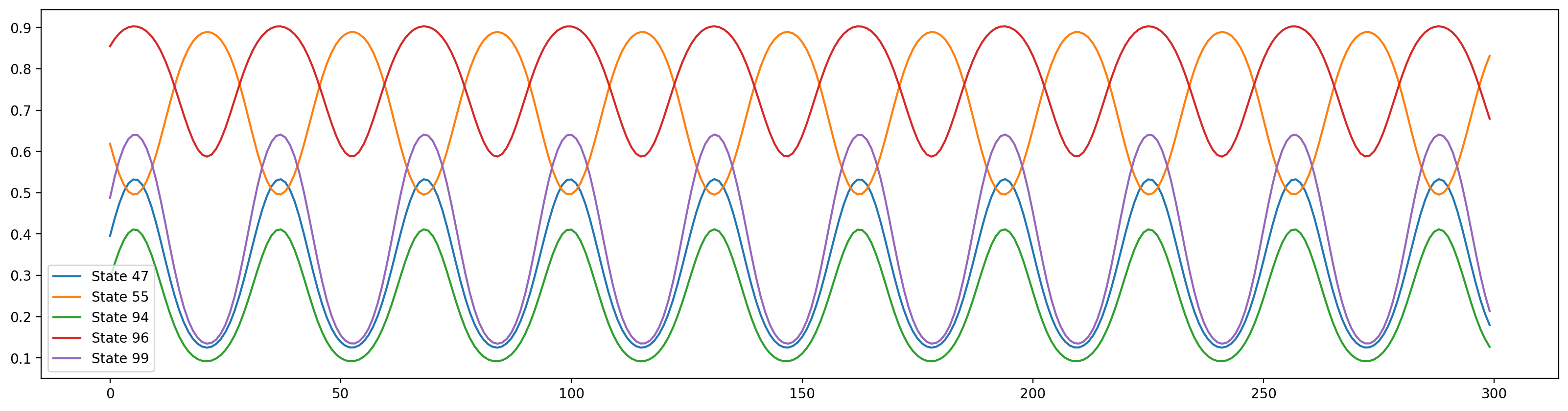
Reservoir Unit States Plot
plt.figure(figsize=(20,5),dpi=200)
randints = np.random.randint(resSize,size=5)
randints.sort()
plt.plot(X_val[randints,:].T)
plt.legend(labels=[f"State {i+1}" for i in randints]);
General case
$x(n+1) = \sigma(\textbf{W}^{in}\cdot u(n+1)_{train} + \textbf{Wx}(n) + \textbf{W}^{back}y(n)_{teach})$
Training
Wback = np.random.uniform(size=(resSize,inSize+1))<0.5
Wback = np.where(Wback==0, -1, Wback)
y_train = 0.5*data[:trainLen]**7

X = np.zeros((resSize,trainLen-initLen))
x = np.random.rand(resSize,1)  #reservoir states random init x(0)
for t in range(1,trainLen):
    u = data[t]
    x = sigmoid( np.dot( Win, np.vstack((1,u)) ) + np.dot( W, x ) + np.dot(Wback, np.vstack((1,y_train[t-1]))))
    if t >= initLen:
        X[:,t-initLen] = x.ravel()

y_train = 0.5*data[initLen:trainLen]**7
Linear Regression
regr = LinearRegression(fit_intercept=False)
with timer("Linear Regression"):
    regr.fit(X.T,np.arctanh(y_train.T))
    Wout = regr.coef_
print(f"MSE train: {np.square(np.dot(Wout,X)-np.arctanh(y_train)).mean()}")
Plot
plt.figure(figsize=(30,2),dpi=200)
incr = 1
plt.plot(range(0,trainLen-initLen,incr),y_train[::incr],'blue',label='Training Data')
plt.plot(range(0,trainLen-initLen,incr),np.dot(Wout,X).ravel()[::incr],'r.',alpha = 0.8,label='Fit');
plt.legend(fontsize=15,loc="upper right");
plt.xlim(0,trainLen-initLen);

Validation
y_pred = np.zeros((outSize,valLen))
X_val = np.zeros((resSize,valLen))
y_val = 0.5*data[trainLen-1:]**7

x = X[:,-1,None]
with timer("RC Forecast time"):
    for t in range(valLen):
        u = data[trainLen+t]
        x = sigmoid( np.dot( Win, np.vstack((1,u)) ) + np.dot( W, x ) + np.dot(Wback, np.vstack((1,y_val[t]))))
        X_val[:,t] = x.ravel()
        y_pred[:,t] = np.tanh( np.dot( Wout, x ) )

y_val = 0.5*data[trainLen:]**7

mse = np.square(y_val - y_pred.ravel()).mean()
print('MSE validation: ' + str( mse ))
Plot
plt.figure(figsize=(30,4),dpi=200)
incr = 1
plt.plot(range(0,valLen,incr),y_val[::incr],'blue',label='Ground Truth')
plt.plot(range(0,valLen,incr),y_pred.ravel(),'r.',alpha = 0.8,label='Prediction');
plt.legend(fontsize=15,loc="lower left");
plt.xlim(0,valLen);

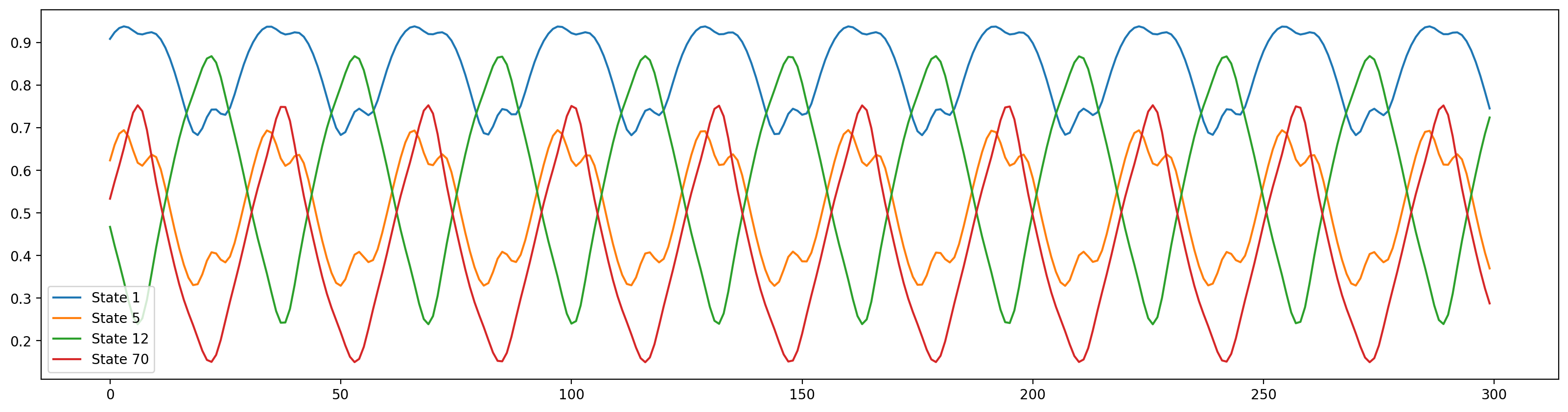
Reservoir Unit States Plot
plt.figure(figsize=(20,5),dpi=200)
randints = np.random.randint(resSize,size=4)
randints.sort()
plt.plot(X_val[randints,:].T)
plt.legend(labels=[f"State {i+1}" for i in randints]);
Comparison with RNN
Importing Tensorflow
import tensorflow as tf
from tensorflow.keras import Model, Sequential
from tensorflow.keras.layers import Dense, Dropout, BatchNormalization, Input, Flatten, LSTM
from tensorflow.keras.optimizers import Adam
from tensorflow.keras.callbacks import EarlyStopping, ModelCheckpoint, ReduceLROnPlateau, Callback, TensorBoard
Create the RNN
model = Sequential()
model.add(LSTM(20, return_sequences=True, input_shape=(1,1)))
model.add(BatchNormalization())
model.add(LSTM(20, return_sequences=False))
model.add(BatchNormalization())
model.add(Dense(10,'relu'))
model.add(BatchNormalization())
model.add(Dense(outSize))
model.compile(optimizer=Adam(lr=0.001), loss='mse')
model.summary()
Training
Optimization Problem: $argmin_{\theta} ||\text{RNN}^\theta(u(n)) - 0.5*u^7(n+1)||,n \in \mathbb{N}_{train}$
class CustomLogger(Callback):
    def __init__(self, epochs_tot):
        super().__init__()
        self.epochs=epochs_tot
        self.threshold = 1000

    def on_epoch_begin(self, epoch, logs=None):
        self.time_begin = time.time()
    def on_epoch_end(self,epoch,logs=None):
        duration = time.time() - self.time_begin
        if (epoch+1) % self.threshold == 0 or epoch==0:
            print(f"The average {self.model.loss} in epoch {epoch+1} is {logs['loss']:1.8f}. Duration: {duration} seconds")

epochs = 10000
batch_size = 301
reduceLR = ReduceLROnPlateau(monitor='loss', factor=0.5, patience=epochs//10, min_lr=1e-7, verbose=1)
earlyStopping = EarlyStopping(monitor='loss', patience=epochs//2)
logger = CustomLogger(epochs)
with timer("RNN Training time"):
    history = model.fit(data[:trainLen,None,None],0.5*data[:trainLen,None,None]**7,batch_size=batch_size,epochs=epochs, verbose=0, callbacks=[earlyStopping,logger])
Plot
plt.figure(figsize=(30,2),dpi=200)
incr = 1
plt.plot(range(0,trainLen,incr),0.5*data[:trainLen][::incr]**7,'blue',label='Ground Truth')
plt.plot(range(0,trainLen,incr),history.model.predict(data[:trainLen,None,None])[::incr],'r.',alpha = 0.8,label='Prediction');
plt.legend(fontsize=15,loc="lower left");
plt.xlim(0,trainLen);

Validation
with timer("RNN Forecast time"):
    RNN_val = history.model.predict(data[trainLen:,None,None])
RNN_mse = np.square(RNN_val-y_val).mean()
print('MSE validation: ', RNN_mse)
Plot
plt.figure(figsize=(30,4),dpi=200)
incr = 1
plt.plot(range(0,valLen,incr),y_val[::incr],'blue',label='Ground Truth')
plt.plot(range(0,valLen,incr),RNN_val[::incr],'r.',alpha = 0.8,label='Prediction');
plt.legend(fontsize=15,loc ="lower left");
plt.xlim(0,valLen);
