Notebook Overview
In this notebook we show the results of the reinforcement learning algorithm described by Briola et al.:
- The agent is allowed to buy/sell/hold at most one unit of Garanti stock at each time step.
The agent can short or long or do nothing (preserve his current position) at each time step. He can also execute a daily stop-loss, where he checks the current P&L and closes all positions and stops further trading in the case of negative total profit.
An environment is a daily Limit Order Book (LOB) environment, containing 5 levels of bid/ask prices/volumes at millisecond precision.
- The states returned by the environment at each time step are the last 10 LOB bars (1 for Echo State Network), the agent's current position (neutral, long or short) and the mark-to-market-value at the current time step.
Possible actions: 'sell','stay','buy', 'daily stop loss'.
The agent is trained using the Proximal Policy Optimization (PPO) algorithm.
Since the agent can possess only one unit of stock at a time, a 'buy' action while in long position would be equivalent to a 'stay' action, whereas a 'sell' action would close the position. Similarly, a 'sell' action while shorting would be equivalent to a 'stay' action, whereas a 'buy' action would close the position.
A difference in this work compared to the original should be noted, which is that our agent trades on mid-prices. In the more realistic scenario, where the spread is taken into account, the agent is not able to generate profit on the dataset at hand but completes the training with a total reward of zero, i.e. there is no net loss or gain.
The agent is trained on the first 60% of the year 2017. Data from the rest of the year (40%) is reserved for validation. Hyperparameters for training were optimized using Optuna.
from IPython.display import HTML
def hide_code(): return HTML('''<script>code_show=true; function code_toggle() {if (code_show){$('div.input').hide();} else {$('div.input').show();}code_show = !code_show} $( document ).ready(code_toggle);</script><form action="javascript:code_toggle()"><input type="submit" value="Click here to toggle on/off the raw code."></form>''')
hide_code()
import sys,os
sys.path.append("./../../")
sys.path.append("./../../../../")
sys.path.append(os.getenv('HOME')+'/#myprojects/')
from Plotter.plotter import plotter
import pandas as pd
import numpy as np
from utils.df_handler import force_zehnerpot
from IPython.display import display, HTML
import pickle

model_dir = "./01_12_21/"

sys.path.append(model_dir)

LOB = pd.read_pickle("../../pkls/LOB_conti.pkl")

dates = pd.unique(LOB.index.date)

validation_dates = dates[len(dates)//10 * 6:]

LOB_on_certain_day = lambda lob,date: lob[lob.index.date == date]
Validation
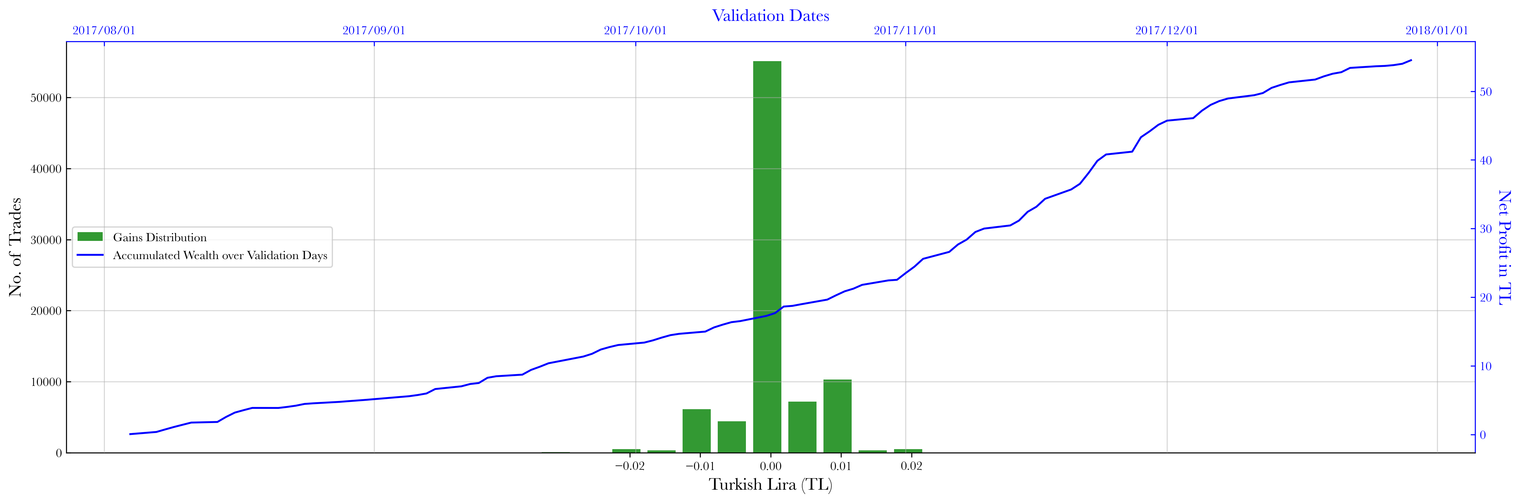
Here we let our trained agent trade on the validation days and look at the P&L.
Model
The model has 2 hidden layers with 64 nodes each, shared by both value and policy networks. Value network's output has length 1. Policy network's output has length 4 for 4 possible actions. These 4 values represent the probability weights passed to a Categorical Distribution.
with open(model_dir+'/model_summary.txt') as f:
    lines = f.readlines()

models_summary=''
line_length=len(lines[0].split('\n')[0])
for line in lines:
    models_summary+= line.split('\n')[0].ljust(line_length) + '\n'

display(HTML(f'<pre>{models_summary}</pre>'))
Rewards
Now we look at the validation performance of our model.
with open(model_dir+"rewards_mid.pkl", "rb") as f:
    rewards_mid = pickle.load(f)

rewards_daily_mid = [*map(sum,rewards_mid.values())]
wallet = np.cumsum(rewards_daily_mid)
total_reward_mid= sum(rewards_daily_mid)
print(f"Total Gains: {round(total_reward_mid,2)} TL in {validation_dates.size} days.")

mcpd = {1:['darkgoldenrod','royalblue'],2:['darkgreen','darkblue']} #model_color_pair_dict
args = [
        [
        [np.concatenate([*rewards_mid.values()]),"rice",dict(color='g',alpha=0.8,label=f"Gains Distribution")],["P&L",dict(fontsize=20,pad=30)],["Turkish Lira (TL)"] ,["#Trades"]
            ,[validation_dates,wallet,dict(color='b',label=f"Accumulated Wealth over Validation Days")],[dict(loc="center left")],[dict(direction='in')]
                        ,dict(color="blue"),[dict(axis='both',colors='blue',direction='in')]
                                ,["%Y/%m/%d"],["Validation Dates",dict(color="blue")],["Net Profit in TL",dict(labelpad=10,rotation=-90,color="blue")]
                                                        ,[dict(b=True,axis='y',alpha=0.5)],[dict(b=True,axis='x',alpha=0.5)]
        ]
]

attrs = ["hist","set_title","set_xlabel","set_ylabel"
             ,"2nd_plot","legend","tick_params"
                     ,"2nd_color_ax","2nd_tick_params"
                             ,"2nd_time_formatx","2nd_set_xlabel","2nd_set_ylabel"
                                            ,"grid","2nd_grid"]
plotter(args,attrs,ncols=1,dpi=300,show=1,second_plot=1);
Training
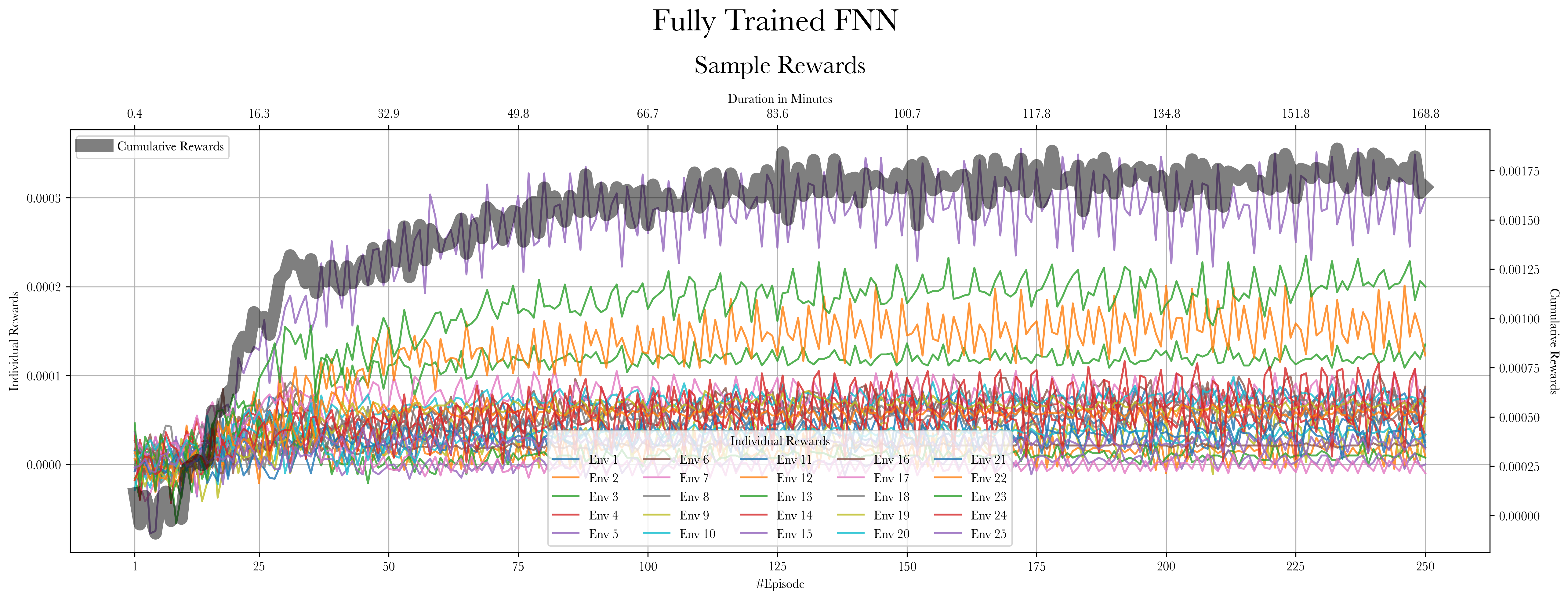
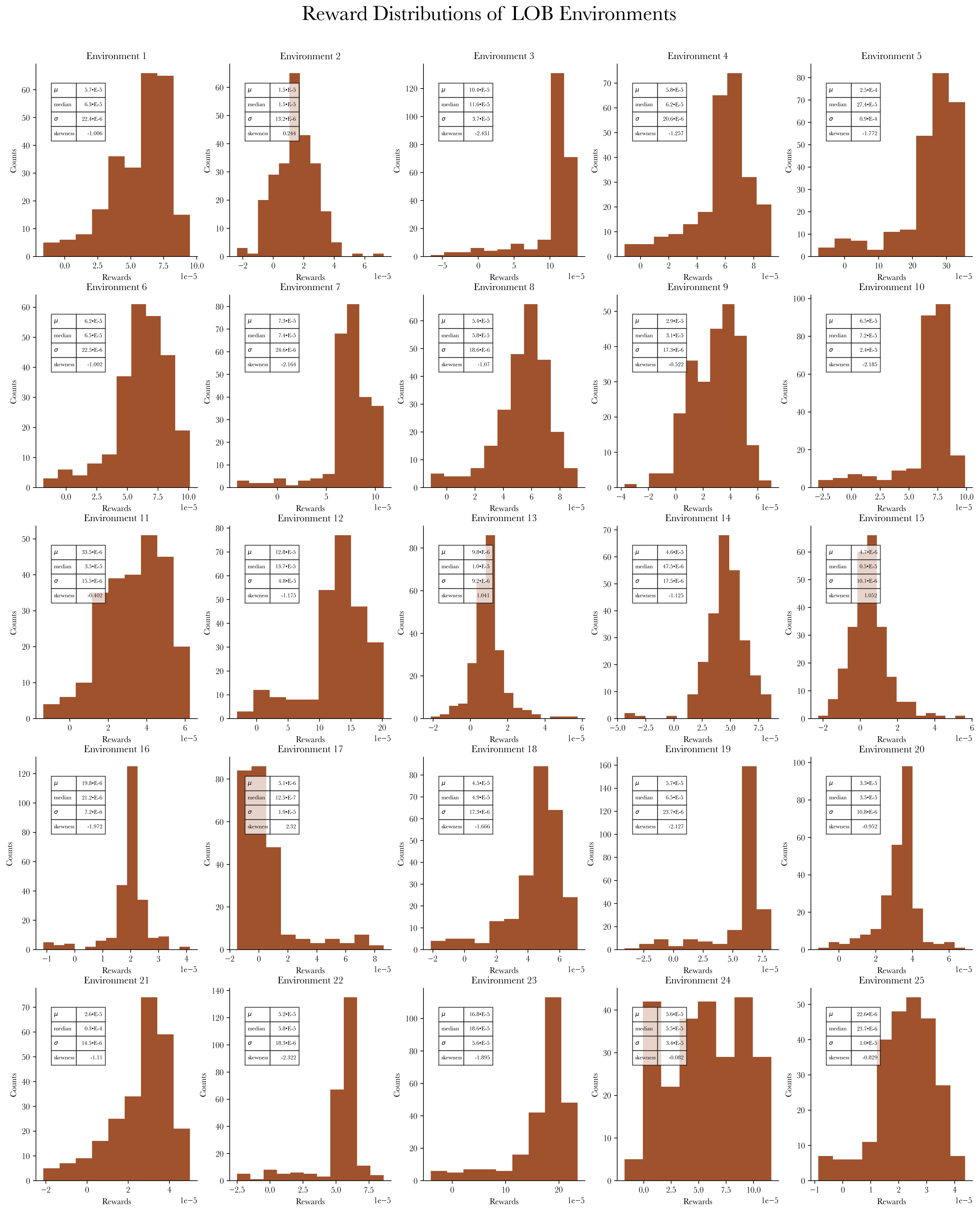
As explained in the data preparation section, we take 25 high signal-to-noise ratio LOB samples and put them inside a vectorized environment to train on.
Mean rewards per PPO episode for each environment can be seen below as well as the distribution of these.
rewards_df = pd.read_csv(model_dir+'rewards_df.csv',index_col=0)

with open(model_dir+'log.txt') as f:
    lines = f.readlines()
    time_elapsed = pd.Series([*map(lambda x: x.split('|')[2].strip() if 'time_elapsed' in x else None,lines)]).dropna().map(int).reset_index(drop=True).divide(60).round(1)
    iterations = time_elapsed.size ; time_elapsed.index += 1

print(f"Training duration: {round(time_elapsed.iloc[-1]/60,2)} Hours, Model taken from iteration no. {len(rewards_df)}, Total iterations: {iterations}.")

means = rewards_df.mean(0).apply(lambda x:force_zehnerpot(x,1,0.01))
medians = rewards_df.median(0).apply(lambda x:force_zehnerpot(x,1,0.01))
stds = rewards_df.std(0).apply(lambda x:force_zehnerpot(x,1,0.01))
skews = rewards_df.skew(0).round(3)

stats = [means,medians,stds,skews]

args = [
        [[(rewards_df.index+1).tolist(),rewards_df,dict(alpha=0.8,markersize=0.01,label=[f"Env {i}" for i in range(1,25+1)])],
                    [rewards_df.index+1,rewards_df.sum(1),dict(linewidth='10',color='k',alpha=0.5,label='Cumulative Rewards')]
                    ,[[1]+rewards_df.index[25::25].tolist()+[rewards_df.index[-1]+1],time_elapsed.loc[[1]+rewards_df.index[25::25].tolist()+[rewards_df.index[-1]+1]].values]
                    ,["Cumulative Rewards",dict(rotation=-90,labelpad=15)],['Duration in Minutes',dict(labelpad=5)],[],
                             ["Sample Rewards",dict(fontsize=20,pad=45)],["#Episode"],["Individual Rewards"],[[1]+rewards_df.index[25::25].tolist()+[rewards_df.index[-1]+1]],
                                    [dict(loc="lower center",ncol=5,title='Individual Rewards')],[dict(b=True,axis='both',alpha=0.9)]]
        ]

plotter(args \
    ,[  "plot",
        "2nd_plot",
        '2nd_set_xticks'
        ,"2nd_set_ylabel",'2nd_set_xlabel',"2nd_legend",
        "set_title","set_xlabel","set_ylabel",'set_xticks'
        ,"legend","grid"] \
        ,ncols=1,dpi=300,show=1,fig_title=f'Fully Trained FNN',suptitle_y=1.1,suptitle_x=0.51,second_plot=1)

args = [
        [
            [rewards_df[str(i)],"scott",{"zorder":0,"color":"sienna"}]
        ,[dict(axis='x', style='scientific',scilimits=(-5,-5))],[f"Environment {i+1}"],["Rewards"],["Counts"]
            ,[dict(cellText=[[stats[0][i]],[stats[1][i]],[stats[2][i]],[stats[3][i]]], rowLabels=[r"$\mu$","median",r"$\sigma$","skewness"], bbox=(0.25,0.6,0.18,0.3)),
              {'fontsize':7,"zorder":10,"alpha":0.1}]
        ] for i in range(25)]

attrs=["hist"
        ,"ticklabel_format","set_title","set_xlabel","set_ylabel"
        ,"make_table"]
plotter(args,attrs,ncols=5,dpi=300,show=1,fig_title="Reward Distributions of LOB Environments",ypad=-6,suptitle_y=0.92);